
Lorem ipsum dolor sit amet, consectetur adipisicing elit. Odit molestiae mollitia laudantium assumenda nam eaque, excepturi, soluta, perspiciatis cupiditate sapiente, adipisci quaerat odio voluptates consectetur nulla eveniet iure vitae quibusdam? Excepturi aliquam in iure, repellat, fugiat illum voluptate repellendus blanditiis veritatis ducimus ad ipsa quisquam, commodi vel necessitatibus, harum quos a dignissimos.
Close Save changesHelp F1 or ? Previous Page ← + CTRL (Windows) ← + ⌘ (Mac) Next Page → + CTRL (Windows) → + ⌘ (Mac) Search Site CTRL + SHIFT + F (Windows) ⌘ + ⇧ + F (Mac) Close Message ESC
In the following example, we illustrate the sampling distribution for the sample mean for a very small population. The sampling method is done without replacement.
In this example, the population is the weight of six pumpkins (in pounds) displayed in a carnival "guess the weight" game booth. You are asked to guess the average weight of the six pumpkins by taking a random sample without replacement from the population.
Weight (in pounds)
Since we know the weights from the population, we can find the population mean.
To demonstrate the sampling distribution, let’s start with obtaining all of the possible samples of size \(n=2\) from the populations, sampling without replacement. The table below shows all the possible samples, the weights for the chosen pumpkins, the sample mean and the probability of obtaining each sample. Since we are drawing at random, each sample will have the same probability of being chosen.
View Full TableSample
Weight
\(\boldsymbol>\)
Probability
We can combine all of the values and create a table of the possible values and their respective probabilities.
\(\boldsymbol>\)
The table is the probability table for the sample mean and it is the sampling distribution of the sample mean weights of the pumpkins when the sample size is 2. It is also worth noting that the sum of all the probabilities equals 1. It might be helpful to graph these values.

An instructor of an introduction to statistics course has 200 students. The scores out of 100 points are shown in the histogram.
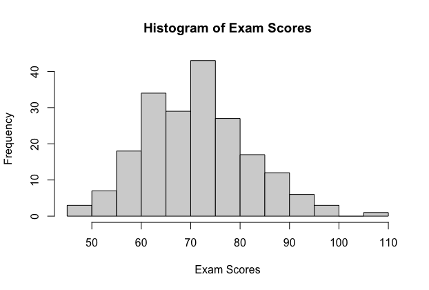
The population mean is \(μ=71.18\) and the population standard deviation is \(σ=10.73\)
Let's demonstrate the sampling distribution of the sample means using the StatKey website. The first video will demonstrate the sampling distribution of the sample mean when n = 10 for the exam scores data. The second video will show the same data but with samples of n = 30.
You should start to see some patterns. The mean of the sampling distribution is very close to the population mean. The standard deviation of the sampling distribution is smaller than the standard deviation of the population.
In the examples so far, we were given the population and sampled from that population.
What happens when we do not have the population to sample from? What happens when all that we are given is the sample? Fortunately, we can use some theory to help us. The mathematical details of the theory are beyond the scope of this course but the results are presented in this lesson.
In the next two sections, we will discuss the sampling distribution of the sample mean when the population is Normally distributed and when it is not.